Computing the betweenness of the doges social network using DNSL method
JJ Merelo
2025-02-21
doges-social-network.RmdIntroduction
Using data from dogesr (Merelo-Guervós 2022), we will, in this
vignette, correct the betweenness centrality of the doges
social network, which was computed using the igraph
package, and therefore does not take into account self-loops. We will
use the dupNodes package (Merelo and
Molinari 2024) to compute the betweenness centrality of the doges
social network, which is a network with self-loops.
Set up
This loads the two involved libraries, as well as loads the data
frame data.doges that contains data on all doges, including
who they married to. Let us see how many self-loops are there
family.marriages <- data.doges[ data.doges$Family.doge == data.doges$Family.dogaressa,]So we have 7 self-loops, including 5 different families. It’s not a lot, but quite enough to make a difference in the status of certain families as expressed by betweenness centrality. These are the families with self-loops:
| Var1 | Freq |
|---|---|
| Candiano | 2 |
| Corner | 2 |
| Faliero | 1 |
| Michiel | 1 |
| Selvo | 1 |
Let’s compute betweenness centrality, with and without self-loops, and see the difference, after extracting only those doges that actually married
library(igraph)
married.doges <- data.doges[ data.doges$Family.dogaressa != '',]
original.betweenness <- betweenness(
  graph_from_data_frame(
    data.frame(married.doges$Family.doge, married.doges$Family.dogaressa), directed=FALSE
    )
  )
dnsl.betweenness <- DNSL.betweenness(
  married.doges,
  first.node="Family.doge",
  second.node="Family.dogaressa")
Which, shown sorted in a table, are:
| x | |
|---|---|
| Dandolo | 446.0000 |
| Contarini | 315.6667 |
| Priuli | 249.3333 |
| Morosini | 243.3333 |
| Loredan | 242.1667 |
| Malipiero | 205.0000 |
| Gradenigo | 199.3333 |
| Mocenigo | 193.5000 |
| Orseolo | 171.0000 |
| Barbarigo | 136.0000 |
| x | |
|---|---|
| Dandolo | 520.6667 |
| Contarini | 375.2667 |
| Priuli | 305.6667 |
| Loredan | 266.7500 |
| Malipiero | 264.0000 |
| Morosini | 263.5000 |
| Mocenigo | 239.5833 |
| Orseolo | 229.0000 |
| Gradenigo | 222.2333 |
| Barbarigo | 148.0000 |
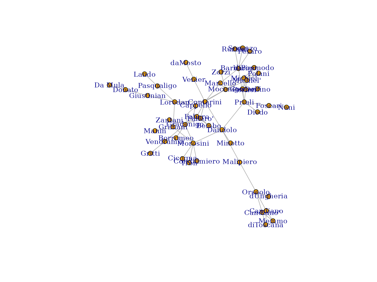
There is some change, due to the fact that there were very few central families, and some of the most prominent had self-loops. The Candiano family was very peripheral, and the change is not enough to make it scale the top 10; the Mocenigo and Gradenigo families have been the one that have changed the most, possibly due to the connection to these families with self-loops. We can see the graph with duplicated nodes here
dup.graph <- dup.nodes.from.data.frame(
  data.frame(V1=married.doges$Family.doge, V2=married.doges$Family.dogaressa)
  )
components <- igraph::components(dup.graph, mode="weak")
biggest_cluster_id <- which.max(components$csize)
vert_ids <- V(dup.graph)[components$membership == biggest_cluster_id]

doges.sn.connected <- igraph::induced_subgraph(dup.graph, vert_ids)
plot(doges.sn.connected,vertex.label.cex=0.9,vertex.size=5)
Conclusions
Intra-family links have its importance in the status achieved by a
family; not only supports its resilience, but also explains the position
they have achieved. This is why it is important to include this new
method to compute betweenness centrality, taking into account not only
the existence of self-loops, but also its value. This
dupNodes package, which is available in CRAN, can be used
to correct betweenness centrality in any eligible network, as well as to
represent the position in the network of these
self-loops-converted-into-duplicated nodes so that it explains whatever
change in the value of centrality or in ranking.